Then the value of the maximum flow in N {\displaystyle N} is equal to the size of the maximum matching in G {\displaystyle G} , and a maximum cardinality matching can be found by taking those edges that have flow 1 {\displaystyle 1} in an integral max-flow.

2. The paths must be independent, i.e., vertex-disjoint (except for s {\displaystyle s} and t {\displaystyle t} ). We can construct a network N = ( V , E ) {\displaystyle N=(V,E)} from G {\displaystyle G} with vertex capacities, where the capacities of all vertices and all edges are 1 {\displaystyle 1} . Then the value of the maximum flow is equal to the maximum number of independent paths from s {\displaystyle s} to t {\displaystyle t} .

To show that the cover C {\displaystyle C} has size n − m {\displaystyle n-m} , we start with an empty cover and build it incrementally. To add a vertex u {\displaystyle u} to the cover, we can either add it to an existing path, or create a new path of length zero starting at that vertex. The former case is applicable whenever either ( u , v ) ∈ E {\displaystyle (u,v)\in E} and some path in the cover starts at v {\displaystyle v} , or ( v , u ) ∈ E {\displaystyle (v,u)\in E} and some path ends at v {\displaystyle v} . The latter case is always applicable. In the former case, the total number of edges in the cover is increased by 1 and the number of paths stays the same; in the latter case the number of paths is increased and the number of edges stays the same. It is now clear that after covering all n {\displaystyle n} vertices, the sum of the number of paths and edges in the cover is n {\displaystyle n} . Therefore, if the number of edges in the cover is m {\displaystyle m} , the number of paths is n − m {\displaystyle n-m} .

Definition. The value of flow is the amount of flow passing from the source to the sink. Formally for a flow f : E → R + {\displaystyle f:E\to \mathbb {R} ^{+}} it is given by:

2. The maximum-flow problem can be augmented by disjunctive constraints: a negative disjunctive constraint says that a certain pair of edges cannot simultaneously have a nonzero flow; a positive disjunctive constraints says that, in a certain pair of edges, at least one must have a nonzero flow. With negative constraints, the problem becomes strongly NP-hard even for simple networks. With positive constraints, the problem is polynomial if fractional flows are allowed, but may be strongly NP-hard when the flows must be integral.[33]

A closure of a directed graph is a set of vertices C, such that no edges leave C. The closure problem is the task of finding the maximum-weight or minimum-weight closure in a vertex-weighted directed graph. It may be solved in polynomial time using a reduction to the maximum flow problem.

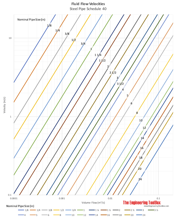
Pipe velocity

In the mentioned method, it is claimed and proved that finding a flow value of k in G between s and t is equal to finding a feasible schedule for flight set F with at most k crews.[29]

Definition. The capacity of an edge is the maximum amount of flow that can pass through an edge. Formally it is a map c : E → R + . {\displaystyle c:E\to \mathbb {R} ^{+}.}

In 2022 Li Chen, Rasmus Kyng, Yang P. Liu, Richard Peng, Maximilian Probst Gutenberg, and Sushant Sachdeva published an almost-linear time algorithm running in O ( | E | 1 + o ( 1 ) ) {\displaystyle O(|E|^{1+o(1)})} for the minimum-cost flow problem of which for the maximum flow problem is a particular case.[10][11] For the single-source shortest path (SSSP) problem with negative weights another particular case of minimum-cost flow problem an algorithm in almost-linear time has also been reported.[12][13] Both algorithms were deemed best papers at the 2022 Symposium on Foundations of Computer Science.[14][15]

To solve this problem one uses a variation of the circulation problem called bounded circulation which is the generalization of network flow problems, with the added constraint of a lower bound on edge flows.

In this method it is claimed team k is not eliminated if and only if a flow value of size r(S − {k}) exists in network G. In the mentioned article it is proved that this flow value is the maximum flow value from s to t.

It was posed to the authors in the spring of 1955 by T. E. Harris, who, in conjunction with General F. S. Ross (Ret.), had formulated a simplified model of railway traffic flow, and pinpointed this particular problem as the central one suggested by the model [11].

In 2013 James B. Orlin published a paper describing an O ( | V | | E | ) {\displaystyle O(|V||E|)} algorithm.[9]

Flow rate calculator

1. In the minimum-cost flow problem, each edge (u,v) also has a cost-coefficient auv in addition to its capacity. If the flow through the edge is fuv, then the total cost is auvfuv. It is required to find a flow of a given size d, with the smallest cost. In most variants, the cost-coefficients may be either positive or negative. There are various polynomial-time algorithms for this problem.

Given a directed graph G = ( V , E ) {\displaystyle G=(V,E)} and two vertices s {\displaystyle s} and t {\displaystyle t} , we are to find the maximum number of paths from s {\displaystyle s} to t {\displaystyle t} . This problem has several variants:

Another version of airline scheduling is finding the minimum needed crews to perform all the flights. To find an answer to this problem, a bipartite graph G' = (A ∪ B, E) is created where each flight has a copy in set A and set B. If the same plane can perform flight j after flight i, i∈A is connected to j∈B. A matching in G' induces a schedule for F and obviously maximum bipartite matching in this graph produces an airline schedule with minimum number of crews.[29] As it is mentioned in the Application part of this article, the maximum cardinality bipartite matching is an application of maximum flow problem.

Remark. Flows are skew symmetric: f u v = − f v u {\displaystyle f_{uv}=-f_{vu}} for all ( u , v ) ∈ E . {\displaystyle (u,v)\in E.}

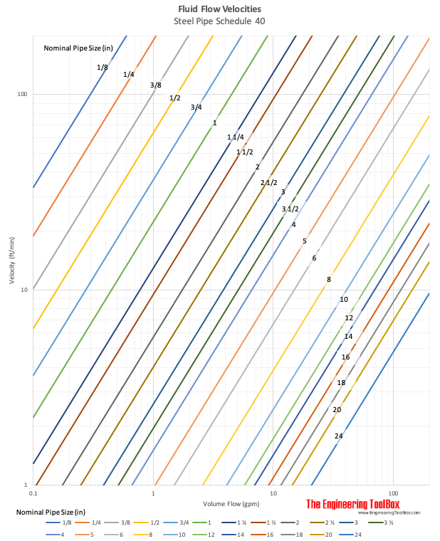
60 US gal/min is flowing through a 4 inch schedule 80 steel pipe . The internal diameter of the pipe is 3.83 in . The velocity can be calculated as

In optimization theory, maximum flow problems involve finding a feasible flow through a flow network that obtains the maximum possible flow rate.

Given a bipartite graph G = ( X ∪ Y , E ) {\displaystyle G=(X\cup Y,E)} , we are to find a maximum cardinality matching in G {\displaystyle G} , that is a matching that contains the largest possible number of edges. This problem can be transformed into a maximum flow problem by constructing a network N = ( X ∪ Y ∪ { s , t } , E ′ ) {\displaystyle N=(X\cup Y\cup \{s,t\},E')} , where

The following table lists algorithms for solving the maximum flow problem. Here, V {\displaystyle V} and E {\displaystyle E} denote the number of vertices and edges of the network. The value U {\displaystyle U} refers to the largest edge capacity after rescaling all capacities to integer values (if the network contains irrational capacities, U {\displaystyle U} may be infinite).

Over the years, various improved solutions to the maximum flow problem were discovered, notably the shortest augmenting path algorithm of Edmonds and Karp and independently Dinitz; the blocking flow algorithm of Dinitz; the push-relabel algorithm of Goldberg and Tarjan; and the binary blocking flow algorithm of Goldberg and Rao. The algorithms of Sherman[6] and Kelner, Lee, Orecchia and Sidford,[7][8] respectively, find an approximately optimal maximum flow but only work in undirected graphs.

Gravitypipeflow calculator

Indeed, for pixels in A (considered as the foreground), we gain ai; for all pixels in B (considered as the background), we gain bi. On the border, between two adjacent pixels i and j, we loose pij. It is equivalent to minimize the quantity

3. In addition to the paths being edge-disjoint and/or vertex disjoint, the paths also have a length constraint: we count only paths whose length is exactly k {\displaystyle k} , or at most k {\displaystyle k} . Most variants of this problem are NP-complete, except for small values of k {\displaystyle k} .[27]

There are some factories that produce goods and some villages where the goods have to be delivered. They are connected by a networks of roads with each road having a capacity c for maximum goods that can flow through it. The problem is to find if there is a circulation that satisfies the demand. This problem can be transformed into a maximum-flow problem.

Let N = ( V , E ) {\displaystyle N=(V,E)} be a network. Suppose there is capacity at each node in addition to edge capacity, that is, a mapping c : V → R + , {\displaystyle c:V\to \mathbb {R} ^{+},} such that the flow f {\displaystyle f} has to satisfy not only the capacity constraint and the conservation of flows, but also the vertex capacity constraint

Definition. The maximum flow problem is to route as much flow as possible from the source to the sink, in other words find the flow f max {\displaystyle f_{\textrm {max}}} with maximum value.

Then it can be shown that G ′ {\displaystyle G'} has a matching M {\displaystyle M} of size m {\displaystyle m} if and only if G {\displaystyle G} has a vertex-disjoint path cover C {\displaystyle C} containing m {\displaystyle m} edges and n − m {\displaystyle n-m} paths, where n {\displaystyle n} is the number of vertices in G {\displaystyle G} . Therefore, the problem can be solved by finding the maximum cardinality matching in G ′ {\displaystyle G'} instead.

Consider a rail network connecting two cities by way of a number of intermediate cities, where each link of the network has a number assigned to it representing its capacity. Assuming a steady state condition, find a maximal flow from one given city to the other.

We now construct the network whose nodes are the pixel, plus a source and a sink, see Figure on the right. We connect the source to pixel i by an edge of weight ai. We connect the pixel i to the sink by an edge of weight bi. We connect pixel i to pixel j with weight pij. Now, it remains to compute a minimum cut in that network (or equivalently a maximum flow). The last figure shows a minimum cut.

In their book, Kleinberg and Tardos present an algorithm for segmenting an image.[32] They present an algorithm to find the background and the foreground in an image. More precisely, the algorithm takes a bitmap as an input modelled as follows: ai ≥ 0 is the likelihood that pixel i belongs to the foreground, bi ≥ 0 in the likelihood that pixel i belongs to the background, and pij is the penalty if two adjacent pixels i and j are placed one in the foreground and the other in the background. The goal is to find a partition (A, B) of the set of pixels that maximize the following quantity

Add standard and customized parametric components - like flange beams, lumbers, piping, stairs and more - to your Sketchup model with the Engineering ToolBox - SketchUp Extension - enabled for use with older versions of the amazing SketchUp Make and the newer "up to date" SketchUp Pro . Add the Engineering ToolBox extension to your SketchUp Make/Pro from the Extension Warehouse !

In 1955, Lester R. Ford, Jr. and Delbert R. Fulkerson created the first known algorithm, the Ford–Fulkerson algorithm.[4][5] In their 1955 paper,[4] Ford and Fulkerson wrote that the problem of Harris and Ross is formulated as follows (see[1] p. 5):

The maximum flow problem was first formulated in 1954 by T. E. Harris and F. S. Ross as a simplified model of Soviet railway traffic flow.[1][2][3]

The claim is not only that the value of the flow is an integer, which follows directly from the max-flow min-cut theorem, but that the flow on every edge is integral. This is crucial for many combinatorial applications (see below), where the flow across an edge may encode whether the item corresponding to that edge is to be included in the set sought or not.

If you want to promote your products or services in the Engineering ToolBox - please use Google Adwords. You can target the Engineering ToolBox by using AdWords Managed Placements.

Given a directed acyclic graph G = ( V , E ) {\displaystyle G=(V,E)} , we are to find the minimum number of vertex-disjoint paths to cover each vertex in V {\displaystyle V} . We can construct a bipartite graph G ′ = ( V out ∪ V in , E ′ ) {\displaystyle G'=(V_{\textrm {out}}\cup V_{\textrm {in}},E')} from G {\displaystyle G} , where

Given a network N = ( V , E ) {\displaystyle N=(V,E)} with a set of sources S = { s 1 , … , s n } {\displaystyle S=\{s_{1},\ldots ,s_{n}\}} and a set of sinks T = { t 1 , … , t m } {\displaystyle T=\{t_{1},\ldots ,t_{m}\}} instead of only one source and one sink, we are to find the maximum flow across N {\displaystyle N} . We can transform the multi-source multi-sink problem into a maximum flow problem by adding a consolidated source connecting to each vertex in S {\displaystyle S} and a consolidated sink connected by each vertex in T {\displaystyle T} (also known as supersource and supersink) with infinite capacity on each edge (See Fig. 4.1.1.).

Assume we have found a matching M {\displaystyle M} of G ′ {\displaystyle G'} , and constructed the cover C {\displaystyle C} from it. Intuitively, if two vertices u o u t , v i n {\displaystyle u_{\mathrm {out} },v_{\mathrm {in} }} are matched in M {\displaystyle M} , then the edge ( u , v ) {\displaystyle (u,v)} is contained in C {\displaystyle C} . Clearly the number of edges in C {\displaystyle C} is m {\displaystyle m} . To see that C {\displaystyle C} is vertex-disjoint, consider the following:

The maximum flow problem can be seen as a special case of more complex network flow problems, such as the circulation problem. The maximum value of an s-t flow (i.e., flow from source s to sink t) is equal to the minimum capacity of an s-t cut (i.e., cut severing s from t) in the network, as stated in the max-flow min-cut theorem.

Let G = (V, E) be a network with s,t ∈ V being the source and the sink respectively. One adds a game nodeij – which represents the number of plays between these two teams. We also add a team node for each team and connect each game node {i, j} with i < j to V, and connects each of them from s by an edge with capacity rij – which represents the number of plays between these two teams. We also add a team node for each team and connect each game node {i, j} with two team nodes i and j to ensure one of them wins. One does not need to restrict the flow value on these edges. Finally, edges are made from team node i to the sink node t and the capacity of wk + rk – wi is set to prevent team i from winning more than wk + rk. Let S be the set of all teams participating in the league and let

Let G = (V, E) be a network with s,t ∈ V as the source and the sink nodes. For the source and destination of every flight i, one adds two nodes to V, node si as the source and node di as the destination node of flight i. One also adds the following edges to E:

where [11] refers to the 1955 secret report Fundamentals of a Method for Evaluating Rail net Capacities by Harris and Ross[3] (see[1] p. 5).

If there exists a circulation, looking at the max-flow solution would give the answer as to how much goods have to be sent on a particular road for satisfying the demands.

We use a third-party to provide monetization technologies for our site. You can review their privacy and cookie policy here.

In the airline industry a major problem is the scheduling of the flight crews. The airline scheduling problem can be considered as an application of extended maximum network flow. The input of this problem is a set of flights F which contains the information about where and when each flight departs and arrives. In one version of airline scheduling the goal is to produce a feasible schedule with at most k crews.

The exact complexity is not stated clearly in the paper, but appears to be E exp ⁡ O ( log 7 / 8 ⁡ E log ⁡ log ⁡ E ) log ⁡ U {\displaystyle E\exp O(\log ^{7/8}E\log \log E)\log U}

In the baseball elimination problem there are n teams competing in a league. At a specific stage of the league season, wi is the number of wins and ri is the number of games left to play for team i and rij is the number of games left against team j. A team is eliminated if it has no chance to finish the season in the first place. The task of the baseball elimination problem is to determine which teams are eliminated at each point during the season. Schwartz[28] proposed a method which reduces this problem to maximum network flow. In this method a network is created to determine whether team k is eliminated.

In other words, the amount of flow passing through a vertex cannot exceed its capacity. To find the maximum flow across N {\displaystyle N} , we can transform the problem into the maximum flow problem in the original sense by expanding N {\displaystyle N} . First, each v ∈ V {\displaystyle v\in V} is replaced by v in {\displaystyle v_{\text{in}}} and v out {\displaystyle v_{\text{out}}} , where v in {\displaystyle v_{\text{in}}} is connected by edges going into v {\displaystyle v} and v out {\displaystyle v_{\text{out}}} is connected to edges coming out from v {\displaystyle v} , then assign capacity c ( v ) {\displaystyle c(v)} to the edge connecting v in {\displaystyle v_{\text{in}}} and v out {\displaystyle v_{\text{out}}} (see Fig. 4.4.1). In this expanded network, the vertex capacity constraint is removed and therefore the problem can be treated as the original maximum flow problem.

Thus no vertex has two incoming or two outgoing edges in C {\displaystyle C} , which means all paths in C {\displaystyle C} are vertex-disjoint.

Note that several maximum flows may exist, and if arbitrary real (or even arbitrary rational) values of flow are permitted (instead of just integers), there is either exactly one maximum flow, or infinitely many, since there are infinitely many linear combinations of the base maximum flows. In other words, if we send x {\displaystyle x} units of flow on edge u {\displaystyle u} in one maximum flow, and y > x {\displaystyle y>x} units of flow on u {\displaystyle u} in another maximum flow, then for each Δ ∈ [ 0 , y − x ] {\displaystyle \Delta \in [0,y-x]} we can send x + Δ {\displaystyle x+\Delta } units on u {\displaystyle u} and route the flow on remaining edges accordingly, to obtain another maximum flow. If flow values can be any real or rational numbers, then there are infinitely many such Δ {\displaystyle \Delta } values for each pair x , y {\displaystyle x,y} .

1. The paths must be edge-disjoint. This problem can be transformed to a maximum flow problem by constructing a network N = ( V , E ) {\displaystyle N=(V,E)} from G {\displaystyle G} , with s {\displaystyle s} and t {\displaystyle t} being the source and the sink of N {\displaystyle N} respectively, and assigning each edge a capacity of 1 {\displaystyle 1} . In this network, the maximum flow is k {\displaystyle k} iff there are k {\displaystyle k} edge-disjoint paths.